Stereogram Pro

A structural analysis platform to optimize all of your analytical workflows. Centered on a spatial-first mindset, all data is easily queryable through spatial selection in the map with advanced filter functionality. Whether you have 100 or 10,000 measurements, Stereogram Pro provides comprehensive analysis with stereonets, rose diagrams, histograms, and 2D/3D scatter plots. Used across structural geology, paleoflow analysis, and kinematic fault analysis through to slope stability analysis, Stereogram Pro provides flexibility through all of your analytical workflows. All data is stored in the cloud and accessible from any computer through the web.

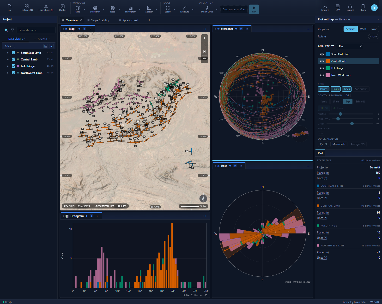
Integrated structural analysis

Comprehensive structural analysis currently requires up to five programs: a stereonet program for plotting and contouring, a spreadsheet program for plots, a third for fault kinematic analysis, a GIS package for map-based analysis, and a data collection app for the field. Stereogram replaces that stack with a single integrated platform.

Stereonet

The core plot, with every projection, contouring method, and orientation statistic you would expect from a dedicated stereonet package.

Capabilities

Equal-area (Schmidt) and equal-angle (Wulff) projections, lower or upper hemisphere
Planes as great circles or poles, plus lineations, slickenlines, and slip arrows on the same plot
Density contouring: Kamb standard, linear, and exponential, plus Schmidt percent-area, with optional Terzaghi bias correction
Fisher and Bingham statistics: mean vectors, confidence cones, and eigenvalue shape parameters
Best-fit great circle and conical (small-circle) fits for fold axes and cone-distributed data
Overlay multiple structural domains or joint sets on one stereonet to compare them directly

Bedding, joints and faults on one stereonet: great circles to poles to Kamb contours, then a cylindrical best fit returning strike/dip, Woodcock K and eigenvalue ratios

Sets picked out by the linked rose diagram carry straight into the stereonet, each contoured on its own colour ramp, then rotate the whole plot to look down any direction

Stereonet of 50 fault planes as great circles with 50 slickenlines drawn as slip arrows, over a linear-method density contour of the fault poles, with a rose inset — Fifty fault planes with their slickenlines drawn as slip arrows, over a linear-method contour of the same poles

Rose Diagram

Azimuthal distributions with real circular statistics behind them, not just petals.

Capabilities

Plot strike, dip direction, trend, or any azimuthal attribute
Adjustable bin width, plotted axially (bidirectional) or directionally
Automatic set detection, or place and adjust sets by hand
Per-set mean direction and von Mises circular statistics with confidence arcs
Full, half, and quarter rose views for datasets confined to one sector

Split the petals by formation, age, site or any attribute; group by age and the wedges take their colours from the ICS chart

Sets found automatically from the distribution, or dragged into place by hand; either way the window, mean and the share left unassigned are reported

Full, half and quarter extents, so data confined to one sector fills the plot instead of leaving most of the circle empty

Histogram

Distribution plots for any measured or derived value in your project.

Capabilities

Dip, plunge, strike, dip direction, trend, rake, elevation, or any custom numeric field
Adjustable bin width with an optional kernel density (KDE) curve over the bars
Per-group colouring so sets and feature types stay separable in a single plot
Summary statistics reported alongside the distribution

The same 5° dip histogram regrouped from feature type to stratigraphic age; narrow it to three ages and each keeps its own KDE curve and summary statistics

A strike histogram of 189 Lower Jurassic planes at 10 degree bins, overlaid with a kernel density curve, a cumulative distribution curve on a second axis, and a dashed circular-mean line at 200 degrees, with circular mean, circular standard deviation, mean resultant and von Mises kappa listed beside the plot — Strike for one age at 10° bins, carrying a KDE, a cumulative curve on its own axis and the circular mean, with R̄ and von Mises κ reported alongside

A grouped strike histogram at 20 degree bins comparing 189 Lower Jurassic planes against 106 Triassic planes, each age drawn in its own colour with its own kernel density curve and dashed circular-mean line, at 201 and 182 degrees respectively — Two ages side by side at 20° bins: each keeps its own density curve and circular mean, 201° for the Lower Jurassic against 182° for the Triassic

2D/3D Scatter

Cross-plot orientation against position, elevation, or your own attributes to find relationships a stereonet alone will not show.

Capabilities

Any pair of attributes on the axes: orientation against latitude, longitude, elevation, or a custom field
Three-axis scatter with a freely rotated camera and a draggable slab for slicing through the cloud
Density clouds and contour overlays that keep trends readable at full dataset size
Selections made here apply everywhere else, so an outlier group can be isolated and inspected on the stereonet or map

Strike against dip for 409 planes, split by feature type: the bedding holds a narrow strike band while the foliation spreads across every azimuth

Recolour the same cross-plot by any continuous field (latitude here) and a spatial gradient reads straight off the points

Latitude, longitude and dip on three axes, orbited freely; a floor projection and distance-scaled points keep the cloud readable while it turns

Cut a section slab through the cloud and drag it along any axis; only the measurements inside stay lit, and the plot reports how many fell outside

Map View

The spatial anchor for the whole project. Every measurement carries its location, and the map is where you query it.

Capabilities

Esri satellite imagery, Esri World Topo, OpenTopoMap, and USGS Topo basemaps
Strike and dip symbols drawn to true orientation with dip-value labels
Lasso and box selection directly on the map, feeding every other plot in the workspace
Define structural domains spatially, then analyse and compare them as separate populations
UTM or latitude/longitude, with tens of thousands of measurements on screen at once

Switch Analyze By to Site and the map symbols, stereonet, histogram and rose recolour together: four limbs of a folded sequence separated in every view at once

4,369 planes and 4,393 lineations over satellite and hillshade; blend the basemap layers and scale the symbols and labels until a dense survey still reads

T axes from 4,352 fault and slickenline pairs, gridded into a regional strain map; grid spacing, search radius and a minimum count per cell decide how far the extension directions are carried

Kinematic Analysis

Fault plane and slickenline pairs resolved into the axes and solutions used to interpret a deformation history.

Capabilities

P, B, and T axes computed from plane and striae pairs
Fault plane solutions with nodal planes and the auxiliary plane
Movement planes and tangent lineation plots
Full slip-sense range: normal, thrust, dextral, sinistral, and the oblique combinations
Averaged focal mechanism across a fault population
Striae snapping to correct field pairs that do not quite lie in the plane

Fault and slickenline pairs resolved into P and T axes: contour the P axes, and the T axes report a Fisher mean with α₉₅ cones and an eigenvalue breakdown

The averaged fault plane solution over the same population, with both nodal planes shaded, P, B and T axes and a separate eigenanalysis of each axis set

Slope Stability Analysis

Kinematic Markland testing of a discontinuity population against a defined slope face, across all three failure modes.

Capabilities

Planar sliding, wedge, and toppling modes on a single overlay
Daylight envelope and friction cone constructed for the slope face you specify
Lateral limit applied so the test stays genuinely kinematic rather than a pole count
Joint set windows, so sets are tested as populations instead of one pole at a time
Wedge intersections generated from discontinuity pairs
Results banded stable, marginal, or high so a slope can be triaged at a glance

Planar sliding overlay: daylight envelope, 30 degree friction cone and lateral limits over three joint sets, with 70 of 207 poles flagged — Planar sliding: daylight envelope, friction cone and lateral limits over the pole population, with the critical zone counted live

Wedge failure overlay: 1122 discontinuity intersections plotted against the slope great circle and friction cone, 137 of them critical — Wedge failure: every discontinuity pair intersected, then tested between the slope face and the friction cone

Flexural toppling overlay: slip limit great circle and lateral limits isolating set C, 56 of 207 poles flagged as high potential — Flexural toppling: the slip limit and lateral limits pick out the steeply back-dipping set on its own

How Stereogram Pro compares

Feature	Stereogram	App A	App B	App C
What each one is
Built for	Capture and full analysis	Desktop plotting	Outcrop recording	Collecting & archiving
Where it runs	Any browser + iPhone app	Windows / macOS install	iOS / Android phone	iOS / Android + web
Interface	Dockable panes, dark mode	Classic desktop	Phone-first	Form-driven
Data structure
Project hierarchy	Sites → stations → measurements	Flat list per file	Localities → measurements	Nested spots
Your own feature types, rather than a fixed list	✓ unlimited	–	Fixed list	Fixed vocabulary
Custom text, numeric and categorical fields on every measurement	✓	–	Notes only	Tags & notes
Named formations with a geologic epoch, coloured from the timescale	✓	–	–	Rock-unit forms
Slickenline stored as a child of its fault plane, so the pair travels together	✓	By row order	Separate record	Same spot
Position, accuracy, declination and quality on every reading	✓	–	Position, declination	Position
Photos on stations and measurements	✓ + annotations	–	✓	✓
Latitude/longitude or UTM, and any EPSG code on import	✓	No coordinates	Lat/long only	Lat/long only
Filtering and querying
Faceted filter panel with live counts: type, formation, age, photo, custom fields	✓	–	–	Tag search
Range filters on the orientations themselves: strike, dip, dip direction, rake, trend, plunge, elevation	✓ 7 fields	–	–	–
Lasso and box selection straight off the map	✓	–	–	–
One selection shared live by every open view	✓	–	–	–
Save a filtered set as a named group, reusable in every tool and plot	✓ analysis sets	–	–	Tags
Editable spreadsheet over the same data	✓ 4 sheets	Text window	–	Web table
Plot types
Stereonet: Schmidt and Wulff, either hemisphere	✓	✓	Preview only	Basic plot
Density contouring: Kamb standard, linear and exponential, plus Schmidt 1% area	4 methods	✓	–	–
Terzaghi bias correction	✓	–	–	–
Rose diagram with automatic set detection and von Mises statistics	✓	Plain rose	–	–
Histogram of any numeric field, with a KDE curve	✓	–	–	–
2D and 3D scatter, freely rotated, with a slab for slicing the cloud	✓	–	–	–
Map view with true-orientation symbols and dip labels	✓ 4 basemaps	External GIS	Capture map	✓
Several plots open at once, linked to one another	✓ dockable	One at a time	–	–
Operations and analysis tools
Structural tools built in	17, in 5 groups	Core set	–	–
Fisher, Bingham and von Mises statistics with α95 / α99 cones	✓	✓	–	–
Cylindrical and conical best fit for fold axes	✓	✓	–	–
Axial-plane finder from two fold limbs	✓	–	–	–
Rotation about any axis, and unfolding with one bedding plane per measurement	✓	Rotation only	–	–
Rotate the stereonet itself: set a viewing azimuth and inclination to look down a fold axis or straight along a fault	✓	–	–	–
Rotate the data, the reference grid, or both together, with contours and set windows following	✓	–	–	–
Two-plane intersection, dihedral angle, bisectors, all-pairs intersections, apparent dip	✓	Core calculations	–	–
Fault kinematics: P-B-T axes, auxiliary plane, focal mechanism, movement plane	✓ built in	Separate program	–	–
Slope stability (Markland): friction cone, daylight envelope, wedge intersections	✓	–	–	–
Every result saved back into the project as editable, re-plottable data	✓	–	–	–
Field capture and sync
Phone-as-compass capture	✓ free app	–	✓	✓
Two-way sync between phone and desk, with conflict review	✓ live	–	File export	Via server
Offline basemaps in the field	✓	–	✓	✓
Import and export
Reads App B and App C field exports, auto-detected	✓	–	–	–
Spreadsheet import (CSV, TSV, Excel, ODS, GeoJSON) with column mapping and value re-mapping	✓	Text file	–	CSV upload
Quadrant, right-hand-rule and dip-direction notation read side by side	✓	One per file	–	–
Georeferenced raster overlay	GeoTIFF	–	Georef. image	Image basemap
Export	PDF, PNG, SVG, CSV, GeoJSON	PDF / EPS	CSV, project file	CSV, archive

Compiled from each product’s current release and published documentation, August 2026. If something here is out of date, tell us and we will correct it.